Downloads :
| Tools > Financial models |
 Numerical Model for Financial Simulation
of Highway PPP Projects
User guide
Main characteristics of the Numerical Financial Model
General
This financial tool is based on the following main criteria:
Sources of highway project funding are:
|
|
| Financial evaluations are calculated using nominal values, based on real values and escalation rates, defined by the user (inflation rate for costs and indexation rate for tolls and revenues). A single sheet, the Assumptions sheet, presents all data used by the model. |
|
| Input ranges are proposed to the user in the Assumptions sheet. The user can select the figure by using an arrow key. |
|
The financial tool integrates subsidies which may be provided by the Contracting Authority during the operating period. Two modes are available for these subsidies.
|
Data Entry
The key data for the model are defined in the assumptions sheet. Data is entered using the arrow keys with data consistency controlled in real time (e.g. coherency between concession life, construction period and operating period).
There are three data types:
- Data related to technical and financial project characteristics

- Data related to the country-specific data (eg economic and fiscal data)

- Data related to financial ratios for the project

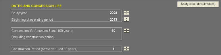
Case study
A case study is defined as the default values in the model. The system is automatically reset with the case study values by pressing the button “Case study” in the sheets “Assumptions”, “Cash Flow graph”, “Debt graph”, “Dividend graph” and “Flux Authority graph”.
General
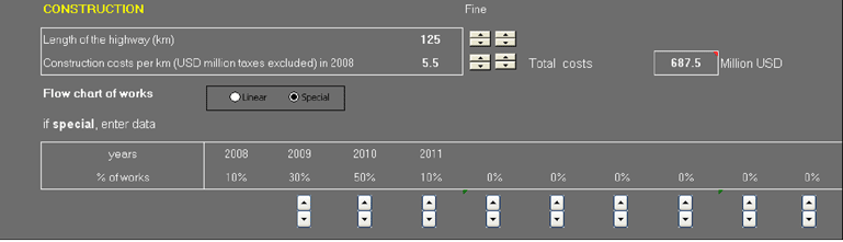
| Length | 125 km of 2x2 lanes |
| Concession duration | 50 years |
| Construction duration | 4 years |
Traffic and Toll
| Categories of vehicles | Light vehicles (70%) - heavy vehicles (30%) |
| Average Daily Traffic at opening | 10,000 vehicles / day |
| Annual Traffic Growth | 3% |
| Toll collected | |
| Category 1 | 0.13 USD / vehicle / km |
| Category 2 | 0.25 USD / vehicle / km |
Construction costs
| Total cost of construction | 5.5 millions USD / km |
Operating costs
| Fixed costs | |||||
| Concessionaire costs (1) | 2 millions USD / year | ||||
| Operation fixed costs | 6 millions USD / year | ||||
| Roadway heavy maintenance costs (2) | 17% of construction cost per 3 years | ||||
| Other maintenance costs | 0.25% of construction cost per year | ||||
| Variable costs (3) | |||||
| Average daily traffic | <=10,000 | >10,000 and <=20,000 | >20,000 and <=30,000 | >30,000 | |
| Costs per vehicle (in USD) | 0.0 | 0.6 | 0.3 | 0.15 | |
Financial structure
| Equity | 10% of the total construction costs | |
| 1st Tranche Debt | ||
| Maturity | 20 years | |
| Interest rate | 4% | |
| Grace period | 5 years | |
| Allocation vs Total debt | 80% | |
| 2nd Tranche Debt | ||
| Maturity | 15 years | |
| Interest rate | 4.5% | |
| Grace period | 6 years | |
| Allocation vs Total debt | 0,1 | |
| 3rd Tranche Debt | ||
| Maturity | 10 years | |
| Interest rate | 6% | |
| Grace period | 6 years | |
| Allocation vs Total debt | 10% | |
| Repayment profile | Annual Debt Service Cover Ratio (ADSCR) = 1.3 used to calculate subsidies | |
| Fees (% of total construction costs) | 1.5% | |
Other
| Type depreciation | Linear |
| Corporate tax | 30% |
| VAT | 19.6% |
| Inflation rate | 2% |
| Discount rate for the sate | 8% |
Comments:
(1) Concessionaire costs: costs of the concession company throughout concession (including construction period).
(2) Roadway heavy maintenance costs: These periodic maintenance works are performed every 8 years but they are considered as annual costs in the financial statements (annual cost = 1/8 of cost).
(3) Variable costs: These costs are dependent on the traffic level according to a regressive scale.
Project periods
Year of study
The year of study corresponds to the current year in which the Project is being assessed, which may be prior to the concession and/or construction period, if so defined. The beginning of operating period corresponds to the year of traffic opening. The beginning of operating period is after the year of study and the construction period.
Concession, Construction and Operation
Concession life: This ranges from 5 to 100 years.
Construction period: A range of 1-10 years is proposed. Construction period is less than or equal to: year of study - beginning of operating period.
Operating period: This is the difference between the concession and the construction period. The operating period immediately follows the construction period. Grace period runs from the start of construction. Operating period begins at the "project year of traffic opening".
Construction costs
The construction costs are calculated from Length of highway and Construction cost per km. They can either be spread linearly over the construction period, or specified each year as a percentage (examples of non linear distributions are proposed).
The construction costs specified are costs in the project study year and exclude VAT. The impact of inflation on construction costs is taken into consideration during the period of construction (“Construction costs in nominal terms”).
Two arrow keys can be used to enter the values:
Length of highway
- the increment of the RH arrow key is 10 km
- the increment of the LH arrow key is 1 km
Construction cost per km.
- the increment of the RH arrow key is 10 Million USD
- the increment of the LH arrow key is 0.5 Million USD
Revenue
Revenues from traffic
The model enables toll levels to be specified for 4 categories of vehicles. These tolls are in USD per km for the Project study year and include VAT.
In the case study, only two toll levels are generated: Category 1 (default value: 0.13USD) and Category 2 (default value: 0.25USD).
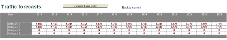
In the same way as for tolls, traffic is split into four vehicle categories. Two profiles can be selected:
- An automatic profile. In this case, three linear growth rates are used to model the traffic increase. The number of years between each growth rate can be changed as required.
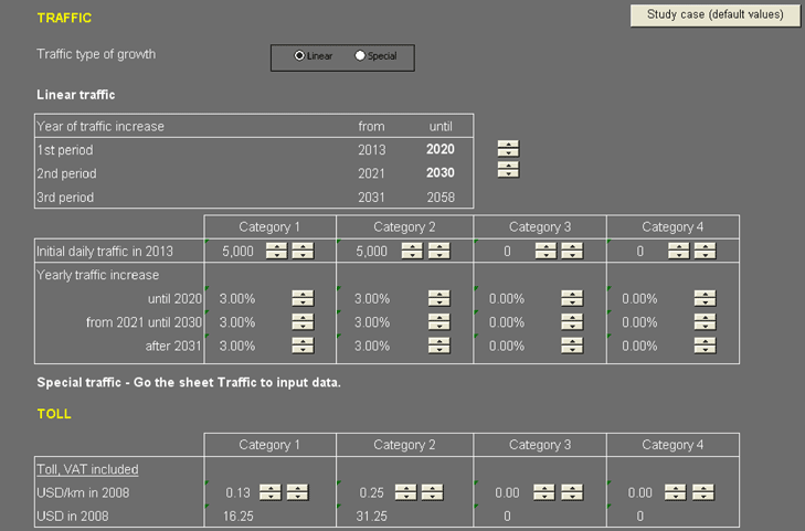
- the increment of the RH arrow key is 0.2 USD per vehicle
- the increment of the LH arrow key is 0.01 USD per vehicle
- A special profile can also be specified by the user by providing the annual daily number of the four categories of vehicles.
In this example, the first growth rate applies to 2020 included, the second rate applies from 2021 to 2030 included and the third rate applies after 2031.
Two arrow keys can be used to enter the toll rates:
Traffic forecasts are input in the TRAFFIC SHEET. The user can generate the linear traffic from the characteristics of “Linear traffic” and then modify the data, or he can input other data. The missing data are generated automatically from the rate of growth of “Linear traffic”.
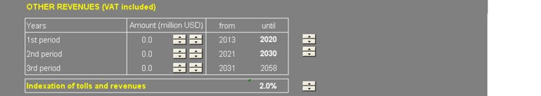
Other revenues
The concessionaire can receive other revenues. Three periods of revenues are possible. For each period, the user enters the amount in real value (value of study year). The revenues are indexed on “index on toll and revenues” (see above).
For example:
- Study year: 2008
- Index on revenues: 3%
- From 2020 to 2030 – revenue: 4 Million USD (in real amount)
- Revenue for 2020 (indexed on “index on revenue” )= 4 x 1.03 2020-2008= 4 x 1.03 12 = 5.703Million USD
Indexation of tolls and revenues
Tolls and revenues are not indexed on inflation, but on a specific index, which can be updated by the user.
Recurrent costs
The operating costs are split in two categories: fixed costs (irrespective of traffic volumes) and variable costs.
Fixed costs
Concessionaire costs
These annual costs cover all the expenses (linked to the management of the concession) of the concessionaire over the entire concession period from the beginning of the construction to the end of concession.
Operation costs
These annual costs are linked to the operation and are incurred by the concessionaire during the operating period (after the construction period). They include personnel costs, administration costs, toll collection costs, etc.
Roadway heavy maintenance costs.
The heavy or periodic road maintenance is performed every ‘n’ (to be specified by the user) years. The amount is a percentage of the construction cost.
Light maintenance costs.
This annual maintenance concerns the routine maintenance of the highway. The amount is a percentage of the construction cost.
Variable costs
The variable costs depend on traffic level and correspond to additional costs resulting from growth in traffic (operation personnel, maintenance, etc.). These costs are estimated as follows:
- From 0 to 10,000 vehicles per day, variable cost = daily traffic x 365 x 0.0 USD
- From 10,000 to 20,000 vehicles per day, variable cost = (20,000 - daily traffic) x 365 x 0.6 USD
- From 20 000 to 30 000 vehicles per day, variable cost = 10 000 x 365 x 0.6 USD + (30 000 - daily traffic) x 365 x 0.3 USD
- If daily traffic > 30 000 vehicles par day, variable cost = 10 000 (veh) x 365 x 0.6 USD + 10 000 x 365 x 0.3 USD + (daily traffic – 30 000) x 365 x 0.15 USD
These costs are increased throughout the concession period at the specified inflation rate.
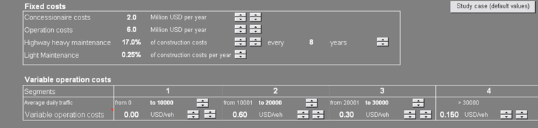
Two arrow keys can be used to enter the rate applied for variable operating costs:
- the increment of the RH arrow key is 0.05 USD per vehicle
- the increment of the LH arrow key is 0.01 USD per vehicle (or 0.005 for tranche 4).
Macroeconomic data
Currency
The model uses Million USD. The 3 tranches of debt are developed in the same currency. Exchange rate issues are not considered in this financial model.
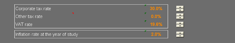
Corporate tax
Corporate tax (profit tax) is paid one year in arrears. The amount of tax is calculated by taking whichever sum is the smaller between (i) the gross profit of the year N and (ii) the cumulated gross profit of the year N.
The corporate tax amount is paid in year N+1.
Other Tax
This rate can be used if VAT is not applied in the user country. Other tax is calculated as a percentage of whole annual toll revenue.
VAT (Value Added Tax)
This rate has a direct influence on the State’s expected revenue as the model assumes that the State’s revenue comes from VAT on each category of vehicle, as repaid by the concession company from the toll revenue.
The model assumes that no road users can reclaim VAT on tolls.
Inflation Rate
The base rate is set at 2% in the model (default value). This rate can be changed by the user.
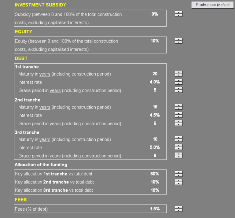
Financial structure
The financial structure of the Concession Company comprises three sources of financing: equity, investment subsidy and debt.
These sources of financing will be used to finance: construction costs, interim interests payments (which will be capitalized and included in debt service), debt fees corresponding to a percentage (specified by the user) of the debt amounts for each year and concessionaire costs.
Equity
The equity is provided by the shareholders of the Concession Company. The user can choose the amount of equity, entered as a percentage of the construction costs.
Investment subsidy
Public Authorities can also provide investment subsidy, also entered as a percentage of construction costs.
Debt
The amount of debt is calculated by the model to reach 100% of investment cost (Equity + Subsidy + Debt = 100% of investment costs). Investment costs include construction costs, capitalised interests, debt fees and concessionaire costs during construction.
Three tranches of debt
The total debt provided to the Project is split into three tranches. Each tranche has its own maturity and interest rate.
The user can specify the allocation of each tranche in the total debt provided to the Project by entering the respective percentages. A tranche whose allocation is equal to 0% will not be drawn.
Interest rates
Three fixed interest rates are available corresponding to the 3 debt tranches.
Grace periods for the tranches
Grace period is the period during which repayment of the principal is deferred; it runs from the start of construction. The grace period is adjusted according to the duration of works (construction period) and is greater or equal to the duration of works.
Repayment profile for the three tranches
The repayment profile of each tranche is on a constant Principal + Interest basis (except for those years within the grace period where the debt is only serviced by the interest paid).
They are repaid at their respective maturities defined by the user in the Assumptions sheet at their respective interest rates.
Fees
The debt fees correspond to a percentage of debt amounts and correspond to the loan management costs.
Financing plan
The three tranches of debt are drawn with the equity and investment subsidy according to their respective schedules to finance the construction costs, capitalized interests and fees during the construction period.
Capitalized interests during the construction period are calculated mid-year.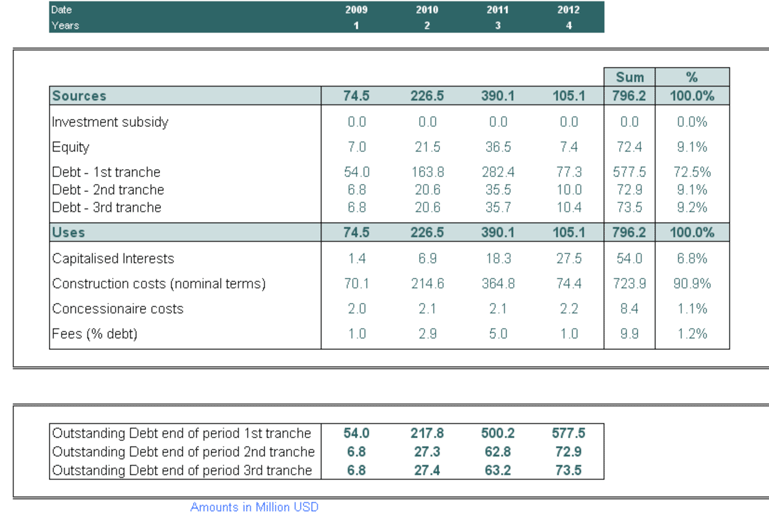
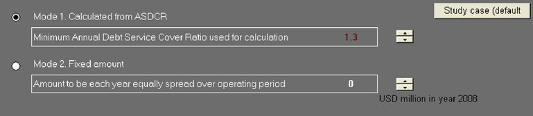
Operating subsidies
If the project’s toll revenue is insufficient to cover its annual operating costs and debt service requirements, annual operating subsidies could be provided to the Project, up to the maximum maturity of the three tranches of debt.
Two modes of calculation of subsidies are available in the Assumptions Sheet in a “mode type” section:
- In Mode 1, subsidies are considered as an output of the financial model.
They are provided to the Project each year when necessary until the final repayment of the three tranches of debt has been made, in order to meet an Annual Debt Service Cover Ratio (ADSCR) defined by the user (Assumptions Sheet – Financial structure) and in accordance with the following formula:
Subsidies = (ADSCR x debt service) + Operating Expenditure – Revenue
NB: If the project’s annual toll revenue is sufficient, subsidies will be set at 0, since the project will have sufficient funds to be financially viable without requiring subsidies.
- In an “input mode” (Mode 2), the user specifies the total amount of subsidies to be provided to the project during the operating period.
In this mode, calculations using the financial tool are based on the total amount of subsidies specified by the user. Subsidies are therefore no longer calculated as in Mode 1, but are fixed by the user.
For calculation purposes, the total amount of subsidies is spread equally over the annual operating period.
Accounting
Distribution of dividends
The amount of distributable reserves in the year N is the sum of retained profits for the year (N-1) and the profit of year N. Whichever is the smallest amount, between the cash balance of the year N and the distributable reserves of year N, is distributed to the shareholders in year N.
The year following the final year of the concession period, all available cash flow for dividends, if any, is distributed between the Concession Company’s Sponsors.
Depreciation
Project assets (i.e. construction costs) as well as capitalized interest during the construction period for the three tranches of debt are depreciated over the operating period. Three types of depreciation are available.
Linear depreciation
The total amount of assets and capitalized interests at the end of the construction period is depreciated annually by the same amount until the end of the concession period.
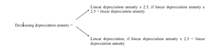
Decreasing depreciation
This type of depreciation is used to benefit the Concession Company in the first years of the concession because the depreciation charge is higher than the linear annuity (the Concession Company therefore pays less corporate tax in the first years of operation if it uses this type of depreciation).
Decreasing depreciation is based on linear depreciation to which a selected factor is applied (2.5 in the financial tool). The calculation is as follows:
Progressive depreciation
This depreciation can be considered as manual depreciation. The operation period is divided in three periods. The user inputs the limit dates of these periods.
- Period 1: One coefficient (<=1) is applied to the linear depreciation
- Period 2: The coefficient applied to the linear depreciation is automatically calculated. It depends on the durations of periods and on the coefficient of the period 1. This coefficient is superior or equal to 1
- Period 3: Linear depreciation is applied.
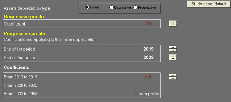
Depreciation throughout the operating period is assumed in the financial tool. Globally, depreciation is linked to the life cycle of the assets which may be shorter than the operating period.
Results
The Annual Debt Service Cover Ratio (ADSCR), Loan Life Cover Ratio (LLCR) and Project Life Cover Ratio (PLCR) are determined throughout the operating period.
Financial ratios
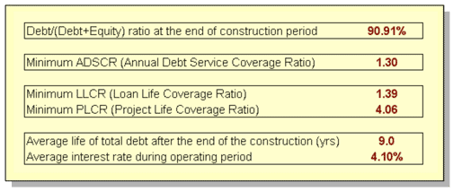
Debt/(Debt +Equity) ratio at the end of the construction period
This ratio is naturally close to the part of debt in the total construction cost.
ADSCR (Annual Debt Service Cover Ratio)
In Mode 1, the ADSCR is used to determine the amount of subsidies in the operating period. In this case, the ADSCR is an input in the model as described in section 9 of this User Guide.
In Mode 2, the ADSCR is a result/output of the model because it is no longer an adjustment variable used to calculate the amount of subsidies required for the Project to be viable. In this mode, subsidies are fixed and the ADSCR will therefore be calculated using the following formula:

where:
i: number of tranches, 1≤ i ≤ 3
n: current year
(Debt Service)i,n = Principali,n + Interesti,n
| CAFDS = Cash Available For Debt Service = | Operating revenue + Other revenues + Subsidy - Fixed operating costs - Variable operating costs - Corporate tax - Other tax + Drawdowns tranche 1 + Drawdowns tranche 2 + Drawdowns tranche 3 |
LLCR (Loan Life Cover Ratio)
The LLCR defined in the financial tool is calculated for the total amount of the debt (i.e. the sum of the three tranches) according to the following formula:

where,
CAFDS corresponds to the above element and
Outstanding debtn end of period to the total amount of the three tranches of debt outstanding at the end of year n.
The Present Value of the Cash Available for Debt Service from year n+1 to the end of the maximum maturity of the three tranches is discounted at an interest rate equal to the weighted average interest rate on the three tranches of debt.
The financial tool provides the user with the minimum LLCR (Results sheet) calculated on the maximum maturity of the three tranches of debt.
PLCR (Project Life Cover Ratio)
The PLCR provided in the model is calculated according to the following formula:

The minimum PLCR is available in Results sheet.
Average life of total debt
The average life of the three tranches of debt is calculated according to the following formula:
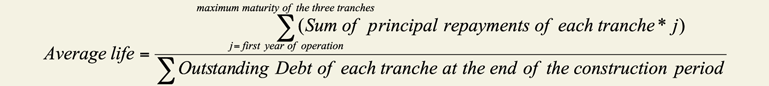
The average life is calculated from the first year of operation.
Average interest rate of the debts
This rate is the average rate of the three tranches of debt.
Shareholder's return
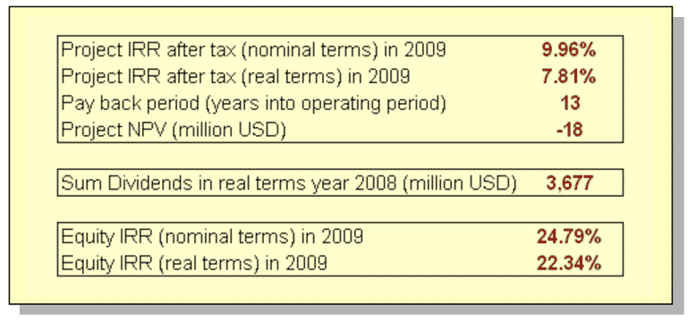
Project IRR
The Project IRR is the rate which satisfies the following formula:

where:
i: number of tranches, 1≤ i ≤ 3
| OCFBF = Operating Cash-Flows Before Financing = | Operating revenue + Other revenues - Fixed operating costs - Variable operating costs - Corporate tax (w/o interests of debts and subsidy) - Other tax. |
This OCFBF does not consider the subsidy and the impact of debt interests and subsidy in the calculation of the corporate tax.
This rate is available in nominal terms and in real terms under the Results Sheet.
PAYBACK period
The payback period is the time taken by a project to recover the initial investment: shorter payback periods are obviously preferable to longer payback periods.
However this method of analysis presents serious limitations because it does not properly account for the time value of money, risk, financing or other important considerations such as the opportunity cost.
Project NPV (Net Present Value)
The operating cash-flows before project financing are discounted at an input discount rate for the state (default value: 8%):

where,
t is the Minimum Project IRR depending upon countries and financial markets.
The NPV is calculated for the first year of the construction period.
Equity IRR (Internal Rate of Return)
This ratio measures the return on investment (equity) for the shareholders. It is calculated for the entire concession period and determined in real and nominal terms for the first year of construction.
The following formula is used to calculate the equity IRR:

where,
Equity injectedi is the equity provided by the sponsors in year i,
Dividendsi are the dividends distributed to shareholders in year i.
Equity IRR is calculated in real terms (through deflated cash flows) and nominal terms (equity - dividends).
Sponsor companies focus on the Equity IRR of the project and compare it to their “hurdle rate”. The hurdle rate represents the rate of return a project must achieve in order to meet investors requirements (minimum acceptable Equity IRR). If the project generates returns in excess of the corporate hurdle rate, it is considered to be financially viable.
Public Authorities financial flows
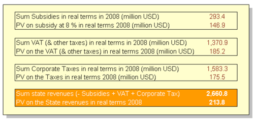
Present Value of subsidies – VAT and Coporate Tax
The total amount of subsidies throughout the concession period is discounted at a real public discount rate defined by the user in the Assumptions sheet.
The PV of the subsidies is calculated for the Project study year using the following formula:

where,
Infl is the inflation rate for the year of study,
r is the discount rate for the State in real terms.
Present Value of VAT
VAT on vehicles will constitute the first source of revenue of the Contracting Authority in the financial tool. The NPV is calculated for the Project study year using the following formula:

where,
Infl is the inflation rate for the year of study,
r is the discount rate for the State in real terms.
Present Value of Corporate tax
Corporate tax will constitute the second source of revenue of the Contracting Authority in the financial tool. The NPV is calculated for the Project study year using the following formula:

where,
Infl is the inflation rate for the year of study,
r is discount rate for the State in real terms.
Limits of daily traffic
The results sheet also gives the minimum and maximum “daily traffic” per category of vehicle over the operating period, i.e. until the end of the concession, as calculated from initial daily traffic and traffic growth rate. These limits allow the user to check traffic with respect to highway capacity or other relevant indicatorsTest on Financial Results
Data inputs can be adjusted in real time using the arrow keys.
The following tests are available to the user under the Results sheet to verify the consistency of results. A general test combining all detailed tests is provided for the user in this sheet. If an error occurs in the detailed tests, this test is negative and a message box appears.
Bankruptcy or financial distress
This test determines whether a Concession Company is bankrupt or in financial distress (terms relate to conditions applicable in beneficiary country).
The test is positive (i.e. company is deemed bankrupt) if the amount of cumulated losses is twice (this coefficient may be modified by the user) the amount of equity. In that case, the year of bankruptcy (or financial distress) is given.
Note: this test relates to conditions applied in France and may not be directly related to the financial strength of a project
Equity IRR calculated > Hurdle rate
The hurdle rate is fixed at 13% in real terms in the financial model. It is assumed that private companies will only participate in the Project if they can obtain an Equity IRR >13%.
If project simulations do not produce such the required level of Equity IRR, the test is negative.
Check Balance Sheet
Check whether the uses and sources of each year of the balance sheet are equal.
Graphic simulation tool
A graphic simulation tool has been added to the numeric model to represent the main financial features of the project in graphic form and their sensitivity to a range of key assumptions. The graphs change in real time to a change in project data.
Four graphs are proposed: Cash Flow Graph, Debt graph, Dividend graph, Flux Authority graph.
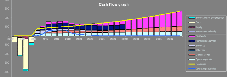
Cash Flow graph
The graph represents all cash flows of the Concession Company during the concession period.
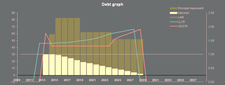
Debt graph
This graph represents separately on the LH and RH axes:
- Annual payments of principal and interest during the debt servicing period (grace period + repayment period)
- Changes in the two main bank ratios over the repayment period: Annual Debt Service Coverage Ratio (ADSCR) and Loan Life Coverage Ratio (LLCR).
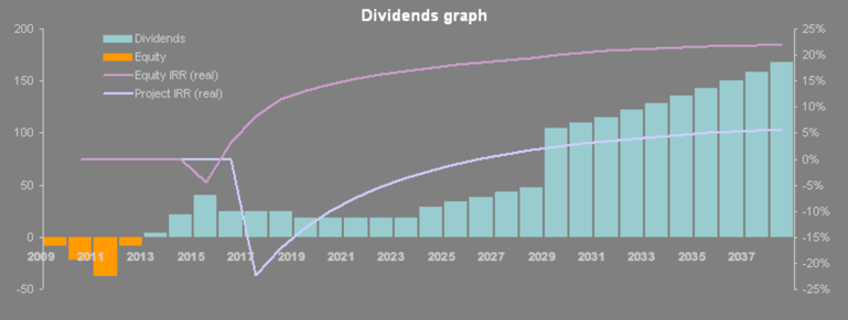
Dividends graph
This Graph displays separately on the LH and RH axes:
- The equity mobilized by company shareholders during the construction period and the dividends received by them during the concession period.
- Changes in the two main investment ratios over the concession: the financial Internal Rate of Return (IRR) of the project and the Equity IRR.
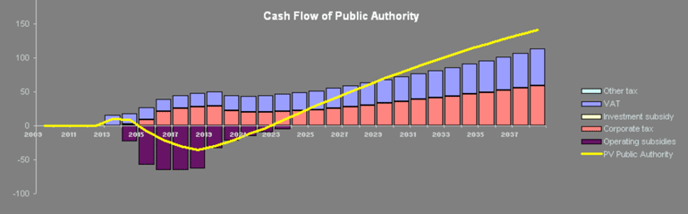
Public authority cash flow graph
The graph represents all cash flows of the Public Authority during the concession period and the NPV of these cash flows.
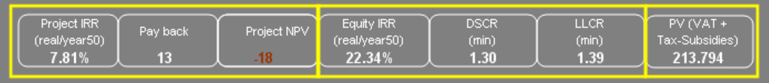
Project indicators & ratios
On each of the four graphs, seven key project indicators / ratios are displayed.
| Project indicators independent of the Financing Plan | |
|
|
| Financing indicators dependent on the Financing Plan | |
|
|
| Public Authorities indicator | |
|
Key project data
Fifteen key assumptions can be modified on each of the three graphs which are automatically adjusted. Ranges of variations have been deliberately limited to realistic values.
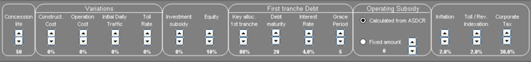
Two types of modifications are possible:
- Enter a new value: concession life, construction period, rate of equity, rate of investment subsidy, first tranche debt, operating subsidy, inflation rate, corporate tax rate
- Enter a variation of the original value: construction cost, operation cost, initial, daily traffic and toll rate.
Summary of project data ranges
The following table describes the lower and upper limits of the main project data.
| Project Data | Minimum | Maximum |
| 1. GENERAL AND CONSTRUCTION | ||
| Study year | 2000 | 2050 |
| Beginning of operating period | Study year +1 | Study year +10 |
| Concession life | Max (5 years; Construction period +1) | 100 years |
| Construction period | 1 year | 10 years |
| Length of highway | 1 km | 1,000 km |
| Construction cost / km | 0.5 Million USD | 200 Million USD |
| 2. TRAFFIC AND TOLL | ||
| Initial daily traffic | 0 vehicle per day | 120,000 vehicles per day |
| Yearly traffic increase | 0% | 100% |
| Toll | 0 USD per km | 20 USD per km |
| 3. OPERATING COSTS | ||
| Fixed costs – concessionaire costs | 0 Million USD | 100 Million USD |
| Fixed costs – operation costs | 0 Million USD | 100 Million USD |
| Fixed costs – highway heavy maintenance | 0% of construction cost | 20% of construction cost |
| Fixed costs – highway heavy maintenance (frequency) | 1 year | 10 years |
| Fixed costs – Light maintenance | 0% of construction cost | 5% of construction cost |
| Variable operation costs (per vehicle) – tr 1 | 0 USD | 2 USD |
| Variable operation costs (per vehicle) – tr 2 | 0 USD | 2 USD |
| Variable operation costs (per vehicle) – tr 3 | 0 USD | 2 USD |
| Variable operation costs (per vehicle) – tr 4 | 0 USD | 2 USD |
| 4. FINANCIAL STRUCTURE | ||
| Equity | 0% | 100% |
| Subsidy | 0% | 90% |
| Debt maturity | Grace period +1 | Concession life |
| Debt – interest rate | 0% | 25% |
| Debt – grace period | Construction period | Debt maturity -1 |
| Debt fees | 0% | 30% |
| 5. DEPRECIATION | ||
| Regressive depreciation coefficient | 1 | 5 |
| Progressive depreciation coefficient | 0.1 | 1 |
| 6. TAXATION & INFLATION | ||
| Corporate tax | 0% | 100% |
| Other tax | 0% | 100% |
| VAT rate | 0% | 100% |
| Inflation rate | 0% | 100% |
| 7. PRIVATE PARTNER | ||
| Minimum Equity IRR in real terms | 8% | 50% |
| Minimum Project IRR in real terms | 10% | 50% |
| 8. PUBLIC AUTHORITIES | ||
| Discount rate for the State in real terms | 2% | 15% |
| 9. MODE OF OPERATING SUBSIDIES | ||
| Minimum Annual Debt Service Cover Ratio | 1.1 | 1.4 |
| Fixed amount | 0 | =Construction_cost/10 |